04. MATLAB Sensor Fusion Guided Walkthrough
MATLAB Sensor Fusion Guided Walkthrough
The following steps will take you on a guided walkthrough of performing Kalman Filtering in a simulated environment using MATLAB. You can download the starter code file
Sensor_Fusion_with_Radar.m
for this walkthrough in the
Resources
section for this lesson.
L4A45 Kalman Tracking+ Walkthru
Project Outline
Radar Sensor Fusion Mini-Project
Project Introduction
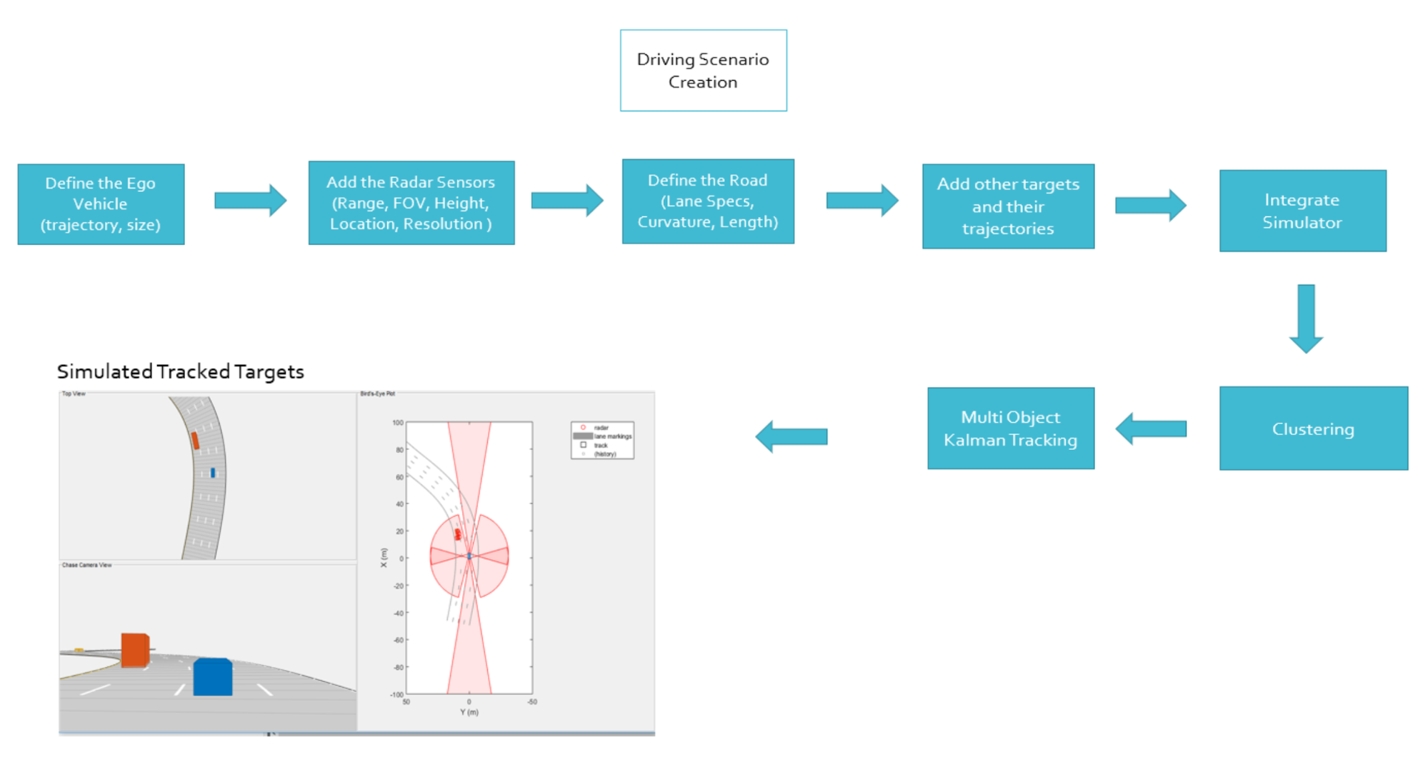
Sensor fusion and control algorithms for automated driving systems require rigorous testing. Vehicle-based testing is not only time consuming to set up, but also difficult to reproduce. Automated Driving System Toolbox provides functionality to define road networks, actors, vehicles, and traffic scenarios, as well as statistical models for simulating synthetic radar and camera sensor detection. This example shows how to generate a scenario, simulate sensor detections, and use sensor fusion to track simulated vehicles. The main benefit of using scenario generation and sensor simulation over sensor recording is the ability to create rare and potentially dangerous events and test the vehicle algorithms with them. This example covers the entire synthetic data workflow.
Generate the Scenario
Generate the Scenario
Scenario generation comprises generating a road network, defining vehicles that move on the roads, and moving the vehicles.In this example, you test the ability of the sensor fusion to track a vehicle that is passing on the left of the ego vehicle. The scenario simulates a highway setting, and additional vehicles are in front of and behind the ego vehicle. Find more on how to generate these scenarios here : Automated Driving Toolbox
% Define an empty scenario

scenario = drivingScenario;
scenario.SampleTime = 0.01;

% Add a stretch of 500 meters of typical highway road with two lanes.
% The road is defined using a set of points, where each point defines the center of the
% road in 3-D space, and a road width.

roadCenters = [0 0; 50 0; 100 0; 250 20; 500 40];
roadWidth = 7.2; % Two lanes, each 3.6 meters
road(scenario, roadCenters, roadWidth);

% Create the ego vehicle and three cars around it: one that overtakes the ego vehicle
% and passes it on the left, one that drives right in front of the ego vehicle and
% one that drives right behind the ego vehicle.
% All the cars follow the path defined by the road waypoints by using the path driving
% policy. The passing car will start on the right lane, move to the left lane to pass,
% and return to the right lane.

% Create the ego vehicle that travels at 25 m/s along the road.
egoCar = vehicle(scenario, 'ClassID', 1);
path(egoCar, roadCenters(2:end,:) - [0 1.8], 25); % On right lane


% Add a car in front of the ego vehicle.
leadCar = vehicle(scenario, 'ClassID', 1);
path(leadCar, [70 0; roadCenters(3:end,:)] - [0 1.8], 25); % On right lane

% Add a car that travels at 35 m/s along the road and passes the ego vehicle.
passingCar = vehicle(scenario, 'ClassID', 1);
waypoints = [0 -1.8; 50 1.8; 100 1.8; 250 21.8; 400 32.2; 500 38.2];
path(passingCar, waypoints, 35);

% Add a car behind the ego vehicle
chaseCar = vehicle(scenario, 'ClassID', 1);
path(chaseCar, [25 0; roadCenters(2:end,:)] - [0 1.8], 25); % On right lane
Define Radar Sensor
Define Radar
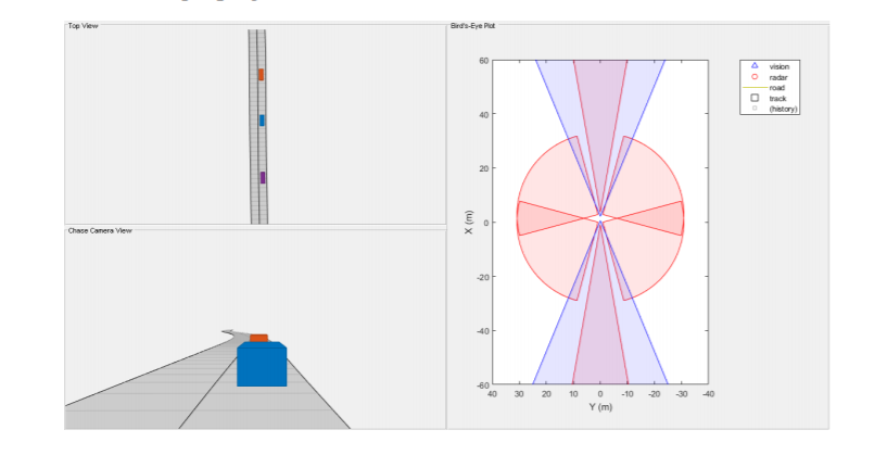
In this example, you simulate an ego vehicle that has 6 radar sensors covering the 360 degrees field of view. The sensors have some overlap and some coverage gap. The ego vehicle is equipped with a long-range radar sensor on both the front and the back of the vehicle. Each side of the vehicle has two short-range radar sensors, each covering 90 degrees. One sensor on each side covers from the middle of the vehicle to the back. The other sensor on each side covers from the middle of the vehicle forward. The figure in the next section shows the coverage.
sensors = cell(6,1);

% Front-facing long-range radar sensor at the center of the front bumper of the car.
sensors{1} = radarDetectionGenerator('SensorIndex', 1, 'Height', 0.2, 'MaxRange', 174, ...
 'SensorLocation', [egoCar.Wheelbase + egoCar.FrontOverhang, 0], 'FieldOfView', [20, 5]);
The rest of the radar sensors are defined in the project code.
Create a Tracker
Create a multiObjectTracker
Create a
multiObjectTracker
to track the vehicles that are close to the ego vehicle. The tracker uses the
initSimDemoFilter
supporting function to initialize a constant velocity linear Kalman filter that works with position and velocity. Tracking is done in 2-D. Although the sensors return measurements in 3-D, the motion itself is confined to the horizontal plane, so there is no need to track the height.
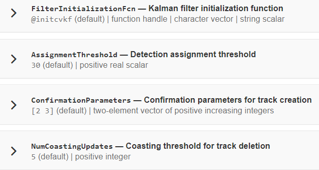
tracker = multiObjectTracker('FilterInitializationFcn', @initSimDemoFilter, ...
 'AssignmentThreshold', 30, 'ConfirmationParameters', [4 5]);

positionSelector = [1 0 0 0; 0 0 1 0]; % Position selector
velocitySelector = [0 1 0 0; 0 0 0 1]; % Velocity selector
MultiObjectTracker Function has several parameters that can be tuned for different driving scenarios. It controls the track creation and deletion One can learn more about these here .
Simulate the Scenario
Simulate the Scenario
The following loop moves the vehicles, calls the sensor simulation, and performs the tracking. Note that the scenario generation and sensor simulation can have different time steps. Specifying different time steps for the scenario and the sensors enables you to decouple the scenario simulation from the sensor simulation. This is useful for modeling actor motion with high accuracy independently from the sensor’s measurement rate.
Another example is when the sensors have different update rates. Suppose one sensor provides updates every 20 milliseconds and another sensor provides updates every 50 milliseconds. You can specify the scenario with an update rate of 10 milliseconds and the sensors will provide their updates at the correct time. In this example, the scenario generation has a time step of 0.01 second, while the sensors detect every 0.1 second.
The sensors return a logical flag,
isValidTime
, that is true if the sensors generated detections. This flag is used to call the tracker only when there are detections. Another important note is that the sensors can simulate multiple detections per target, in particular when the targets are very close to the radar sensors. Because the tracker assumes a single detection per target from each sensor, you must cluster the detections before the tracker processes them. This is done by implementing clustering algorithm, the way we discussed above.
toSnap = true;
while advance(scenario) && ishghandle(BEP.Parent)
    % Get the scenario time
    time = scenario.SimulationTime;

    % Get the position of the other vehicle in ego vehicle coordinates
    ta = targetPoses(egoCar);

    % Simulate the sensors
    detections = {};
    isValidTime = false(1,6);
    for i = 1:6
        [sensorDets,numValidDets,isValidTime(i)] = sensors{i}(ta, time);
        if numValidDets
            detections = [detections; sensorDets]; %#ok<AGROW>
        end
    end

    % Update the tracker if there are new detections
    if any(isValidTime)
        vehicleLength = sensors{1}.ActorProfiles.Length;
        detectionClusters = clusterDetections(detections, vehicleLength);
        confirmedTracks = updateTracks(tracker, detectionClusters, time);

        % Update bird's-eye plot
        updateBEP(BEP, egoCar, detections, confirmedTracks, positionSelector, velocitySelector);
    end

    % Snap a figure for the document when the car passes the ego vehicle
    if ta(1).Position(1) > 0 && toSnap
        toSnap = false;
        snapnow
    end
end
Kalman Filter
Define the Kalman Filter
Define the Kalman Filter here to be used with
multiObjectTracker
.
In MATLAB a
trackingKF
function can be used to initiate Kalman Filter for any type of Motion Models. This includes the 1D, 2D or 3D constant velocity or even constant acceleration. You can read more about this
here
.
initSimDemoFilter
This function initializes a constant velocity filter based on a detection.
function filter = initSimDemoFilter(detection)

% Use a 2-D constant velocity model to initialize a trackingKF filter.
% The state vector is [x;vx;y;vy]
% The detection measurement vector is [x;y;vx;vy]
% As a result, the measurement model is H = [1 0 0 0; 0 0 1 0; 0 1 0 0; 0 0 0 1]

H = [1 0 0 0; 0 0 1 0; 0 1 0 0; 0 0 0 1];
filter = trackingKF('MotionModel', '2D Constant Velocity', ...
 'State', H' * detection.Measurement, ...
 'MeasurementModel', H, ...
 'StateCovariance', H’ * detection.MeasurementNoise * H, ...
 'MeasurementNoise', detection.MeasurementNoise);
end
Clustering
Cluster Detections
This function merges multiple detections suspected to be of the same vehicle to a single detection. The function looks for detections that are closer than the size of a vehicle. Detections that fit this criterion are considered a cluster and are merged to a single detection at the centroid of the cluster. The measurement noises are modified to represent the possibility that each detection can be anywhere on the vehicle. Therefore, the noise should have the same size as the vehicle size. In addition, this function removes the third dimension of the measurement (the height) and reduces the measurement vector to
[x;y;vx;vy]
.
We already went through its implementation in the clustering concept of this lesson.
Project
Run Your Code
Now, It’s time to run the code and see the output!
It is highly recommended to spend some time on this sensor fusion code. It’s a good place to start learning and implementing sensor fusion techniques.
Solution
Workspace Lesson 5